Longitudinal boxplots: statistical summaries and visual conventions

The implemented figure summarizes one confirmed numeric analysis variable across ordered visits, with a separate facet for each selected treatment. Statistical calculations happen before rendering. The plot draws those calculated values directly, so ggplot2 does not choose a second quartile or whisker definition.

View in Full Screen

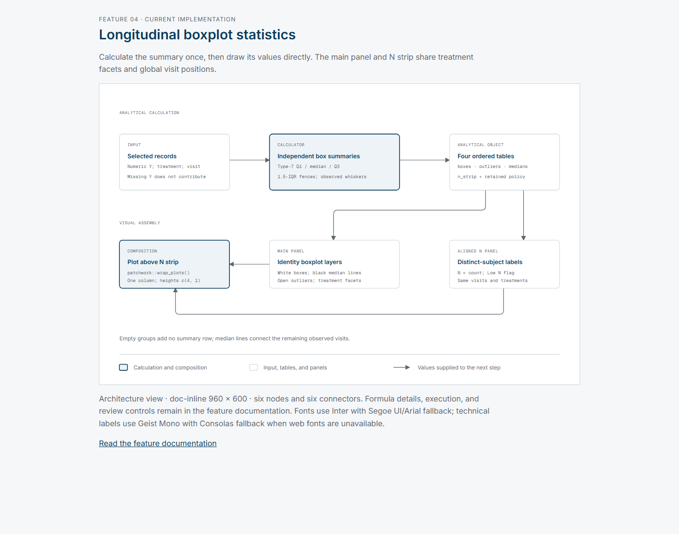
Selected records and grouping

calculate_boxplot_statistics() consumes records from a validated selected-data profile, the treatment and Y column names, ordered treatment and visit levels, and a retained low-N policy. Required columns are USUBJID, AVISIT, AVISITN, the selected treatment column, and the selected numeric Y column. The supported workflow selects stored AVAL, CHG, or PCHG; this calculator does not derive change or percentage change.

The calculator excludes missing Y values, missing treatments, missing visits, and records outside the selected treatment and visit levels. Selected non-finite values cause an error. It orders included records by the supplied treatment order, visit order, and subject identifier, then groups by treatment and visit. Supplied level order controls display positions; AVISITN is retained in analytical rows. Upstream profiling owns visit mappings and duplicate-key checks.

The Y distribution uses included records. The displayed N counts distinct USUBJID values among those records, including records classified as outliers. N therefore describes subjects contributing non-missing selected Y values at that treatment and visit, rather than the number uploaded or the number represented by the box’s interior.

Exact statistical definitions

For sorted values x[1], ..., x[n], the type-7 quantile at probability p uses h = (n - 1) * p + 1. With j = floor(h) and g = h - j, the result is x[j] + g * (x[j + 1] - x[j]); an integer position returns x[j] directly. The calculator applies this definition at 0.25, 0.5, and 0.75 for the lower hinge, median, and upper hinge.

IQR = Q3 - Q1. The inclusive fences are Q1 - 1.5 * IQR and Q3 + 1.5 * IQR. Whiskers end at the smallest and largest observed values inside those fences, rather than at the fence values. Values strictly outside are retained as individual outlier rows, with subject identity, treatment, visit, and value.

The expected-statistics fixture makes small samples and edge cases explicit. For values 1, 2, 3, 20, Q1 is 1.75, the median is 2.5, Q3 is 7.25, whiskers are 1 and 3, and 20 is an outlier. For 5, 5, 5, 5, 10, IQR is zero: both whiskers remain at 5 and 10 is an outlier. A single contributing value produces identical hinges, median, and whiskers.

Low N is a flag, not a filter. It is true when distinct-subject N is strictly below the retained policy value. validate_bds_profile() supplies a default threshold of 5; a non-default policy retains its value, rationale, authority, and version. Labels are N = <count> or N = <count> - Low N. Boxes remain visible when flagged.

Empty groups and connected medians

The boxplot_analysis object retains four tables: boxes, outliers, medians, and n_strip, plus ordered levels, variable names, policy, and analysis_version. An empty treatment-visit combination creates no box, median, or N-strip row. The renderer retains global visit positions and selected facets through factor levels and drop = FALSE; it does not manufacture an N = 0 label.

Median lines connect the remaining observed visit medians within each treatment. If the middle visit has no contributing values, the line connects the surrounding observed visits across that empty position. This is a connection between group summaries, not an individual-subject trajectory or an imputed intermediate median.

Rendering and composition

assemble_boxplot() uses geom_boxplot(stat = "identity") with the five calculated statistics. It disables the geometry’s own outlier drawing and adds retained outliers as open circles. Boxes have white fill and black outlines. Median connections are black lines with larger white-filled circular markers; outliers use smaller open circles.

Treatment facets use grey headers, black panel borders, bold text, pale major grid lines, and no minor grid. The Y label is the selected column name with the selected unit appended when present. The main panel hides visit labels and X ticks; the aligned N strip supplies the Analysis Visit axis. Both panels use identical ordered treatment and visit factors. patchwork::wrap_plots() stacks them in one column with relative heights c(4, 1).

Fixed and free Y scales change the facet scale configuration, not these statistics. Fixed assembly starts at Draft; free assembly starts at Experimental/Draft with a cross-facet comparison warning. Those initial labels do not establish execution verification or human approval.

Implementation evidence and limits

The standalone helpers in boxplot_standalone.R repeat the calculation and visual conventions inside scripts emitted by compile_boxplot_script(). Changes to statistical or visual rules need corresponding scrutiny in both implementations.

Inspected tests cover statistics, assembly, and compiled scripts: explicit fixture results, empty groups, non-finite rejection, row-order invariance, layer values, N-panel alignment, scale differences, and standalone analytical results. The long-label test checks PNG creation and dimensions; it does not establish label legibility through visual inspection. Fixture rows still carry pending_human_review.

This documentation records inspected implementation and test assertions. No R tests, statistical review, or formal validation were run for this documentation change. The diagram describes data flow and omits rendering dimensions, script setup, execution, and review controls, which have separate documentation.